How To Change Chart Style In Excel 2013

How to Change Chart Way in Excel? (Pace past Step)

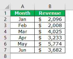
Assume you have a information fix similar the below ane.

You can download this Change Chart Style Excel Template here – Change Chart Manner Excel Template

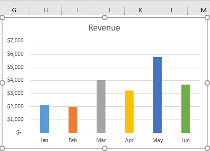
Pace 1 – We must select the data and insert the COLUMN chart in excel Column chart is used to represent data in vertical columns. The height of the cavalcade represents the value for the specific data serial in a chart, the cavalcade chart represents the comparison in the form of column from left to correct. read more .

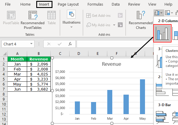
We become this default chart when inserting the column chart for the selected data range. Nonetheless, almost people practice non go across this step because they do not intendance about the dazzler of the chart.

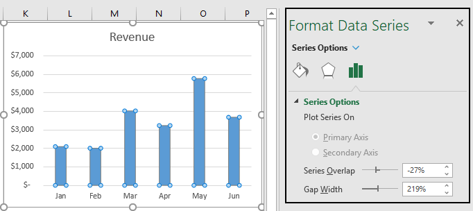
Pace 2 – To open the "FORMAT DATA Series" option, we must select the confined and press "Ctrl + 1."

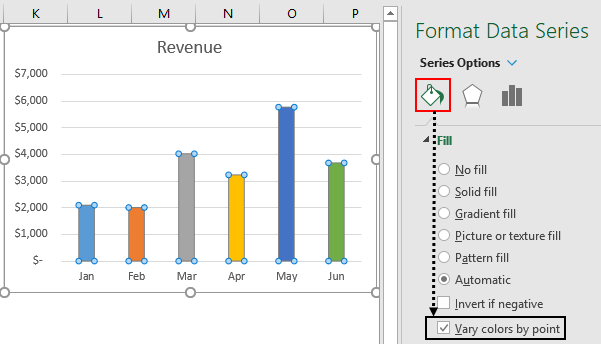
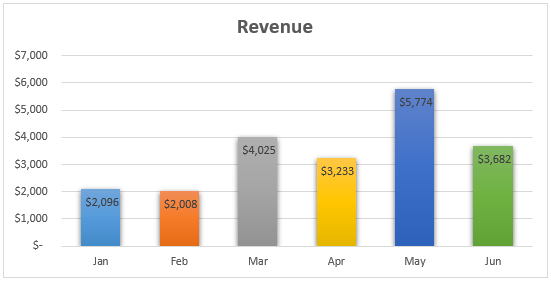
Step iii – In the "FORMAT Data SERIES" window, choose the "FILL" option, click on "Fill," and check the box "Vary color by point."

Steps to Apply Different Themes or Styles to The Chart

Nosotros demand to employ some themes or unlike styles to the chart. For this, we need to follow the below simple steps.

Step i: First, we must select the chart first.
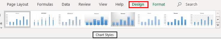
Stride two: 2 extra tabs open up on the ribbon as presently as we choose the chart.

We can see the master heading every bit "Nautical chart Tools," and under this, we have two tabs, i.e., "Pattern" and "Format."

Step 3: We must become to the "DESIGN" tab. Under this, we tin come across many design options. Next, get to the "Chart Style" section.

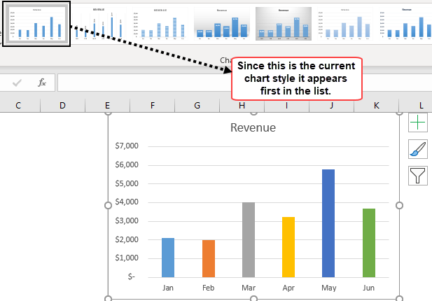
Step 4: As we tin see under "Chart Styles," we tin see many designs. As per our current chart manner, the outset one will appear.

In Excel 2013, nosotros accept a total of sixteen chart styles. So, click on the drop-down list of the chart style to see the list.

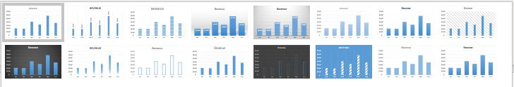
At that place is no specific name for each nautical chart style. Rather, these styles are referred to equally "Way 1", "Style 2", "Fashion 3," then on.

We will come across each style of how they look when we apply them.

Style 1: Utilize only Grid Lines.

If we choose the first way, it will display simply GRIDLINES in excel Gridlines are little lines fabricated of dots to split up cells from each other in a worksheet. The gridlines have slight faint invisibility; you can find it in the page layout tab. This pick has a checkbox; for activating the gridlines, you can tick on information technology and untick if y'all wish to deactivate gridlines. read more to the chart. Below is the preview of the same.

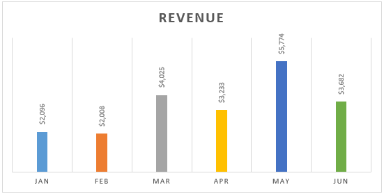
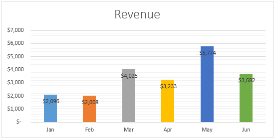
Style two: Show Information Labels in a Vertical way

"Data Labels" are the information or numbers of each column bar. Suppose we select the "Style 2″ choice. We will get beneath the chart style.

Style 3: To Apply Shaded Column Confined

This style volition alter the style of the bars from manifestly to shades. Below is the preview of the same.

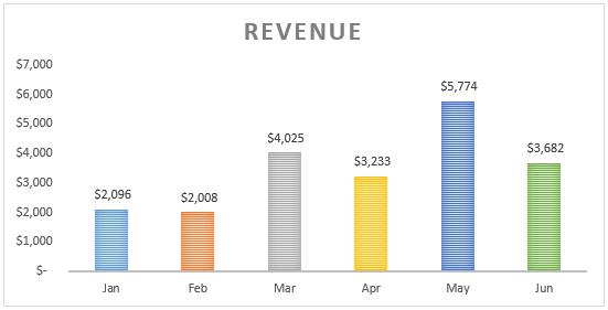
Note: "Information Labels" exercise not default in this mode since we accept selected "Style ii" in the previous step; it has come up automatically.

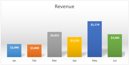
Style 4: To Apply Increased Width of Column Confined and Shadow of Column Bars.

This style will increase the width of the cavalcade confined and give each column bar's shadow.

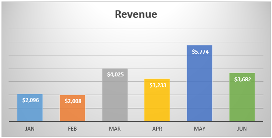
Way v: To Apply Gray Background.

This style will apply a grey background to "Style 4."

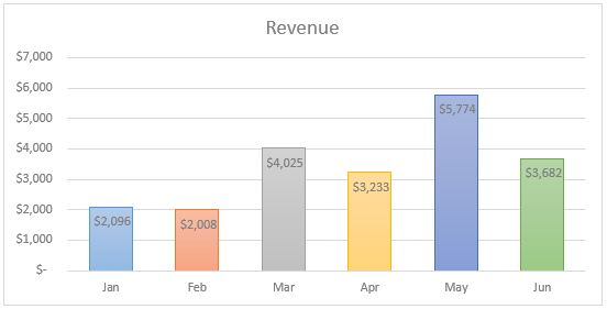
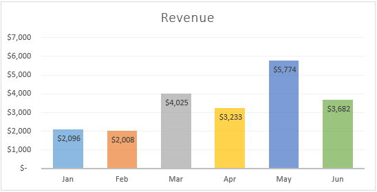
Style 6: To Apply Light Color to the Column Bars.

This style volition apply lite colors to the column bars.

Style vii: To Use Light Gridlines.

This style volition utilise light grid lines to the chart.

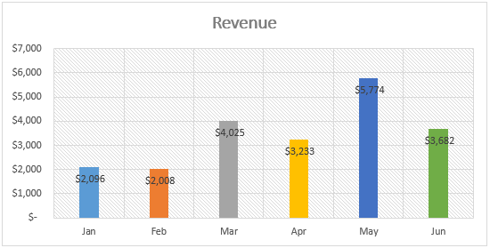
Style viii: To Apply rectangular Gridlines.

This manner will apply a rectangular box type of gridlines with shades.

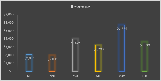
Style 9: To Apply Blackness Background.

This way will apply a dark black colored background.

Fashion 10: To Apply Smoky Lesser to the Column Confined.

This style volition employ the bottom of each column bar as smoky.

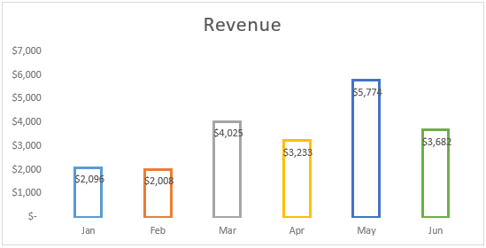
Style eleven: Utilize only borders to the Column Bars.

This style will apply only outside borders to the column bars.

Fashion 12: Similar to Style 1.

This style is like to "Style ane."

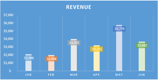
Style 13: To Apply Classy Style Type one

This style volition make the chart more beautiful, as shown beneath.

Style 14: To Use Classy Mode Blazon 2

This style volition make the chart more than beautiful as below.

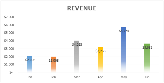
Style xv: To Utilize Increased bar without Gridlines

This style will remove gridlines but increase the width of the column bars.

Manner 16: To Apply Intense Effect to the Cavalcade Bars

This style will use the "Intense Issue" to the column bars.

Things to Remember

Each style is different from the others.
Ever cull elementary styles.
Never go beyond fancy styles, particularly in business presentations.

Recommended Manufactures

This article is a guide to Change Nautical chart Style in Excel. Here, nosotros discuss how to change the chart style in Excel, examples, and a downloadable Excel template. You lot may also look at these useful manufactures in Excel: –

Blitheness Chart in Excel
Table Styles in Excel
Add Filter in Excel
Tornado Chart in Excel

Source: https://www.wallstreetmojo.com/change-chart-style-in-excel/

Posted by: mcdanielmorly1947.blogspot.com